Major results

Isometric embedding analysis for black hole spin

The integration of GCM and frame equations gives good results for metric calculation particularly in the case of \(a\leq a_{\rm lim} = \sqrt{3}/2\). Beyond this limiting value \(a_{\rm lim}\), from computational reasons, we had to shrink down the initial set but we succeed to get the embedding near the equatorial axis for spin \(a<0.99999\).

It is very likely that the \(\mathcal{C}^3\) isometric embedding of Kerr poloidal sub-manifold in the 3-dimensionnal Euclidean ordinary space (like for Kerr black hole horizon cite{PhysRevD.7.289}) could not exist in a global way beyond the limiting value \(a_{\rm lim}\). Besides, we showed that the ergoregion volume increase in function of $a$ is mainly due to the length increase of the equatorial axis inside ergosphere and the ergoregion surface on the embedding.

~

The numerical integration of GCM equations systematically diverges to infinity near the region where the Gaussian curvature gets null. It explains why we need to slice our domain to avoid infinite values. For $a=0.86$, which is the last two-digit precision computed value where we could get the solution without slicing our domain, the values $L(0,pi/2)$, $N(0,pi/2)$ and $M(0,pi/2)$ are close to $0$.

below \(a_{\rm lim}\)

From the left to the right, the isometric embedding in the 3D Euclidean space for $a=0$, $0.5$ and $0.86$. In green the equatorial axis ($lambda=0$), in black the polar axis $(lambda=pmpi/2)$, in red the ergosphere and in blue the horizon.

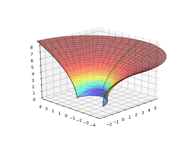
Obtain embedding for \(a = 0.5\). In green the equatorial axis (\(\lambda = 0\)), in polar axis (\(\lambda = ±\pi)\), in red the ergosphere and un blue the horizon.

greater than \(a_{\rm lim}\)

In order to obtain the isometric embedding, we have worked on the sub-domain $mathcal{U}_{s_{rm max}}^{a,f}=left{(s,lambda)inmathcal{U}_{s_{rm max}},|, r^2(s)-3fa^2sin^2lambda>0right}$. For $f=1.27$ we are able to obtain the solutions for $ain [0.86,0.99999]$.

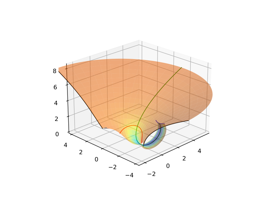
On Fig.(ref{fig-evolutionplongamen-a-0.99-0.99999}), we can observe the coiling of the ergoregion as $a$ increases toward $1$. This coiling is visible only for values of $a$ extremely close to $1$.

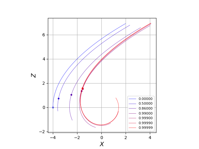
The coiling of the equatorial axis on the left of Fig.(ref{fig-evolveequatorialaxis}) is entirely determined by the choice of the initial conditions in Eq.(ref{Eq-BoundaryCondition-3}). This coiling gets a nearly constant principal curvature along $s$ on the equatorial line when $s$ is close to $0$. When $arightarrow 1^{-}$, the equatorial line is coiling around a circle of radius ${sqrt{2}}$. We already noticed (see Fig.(ref{fig-evolutionangleprimitif})), that the angle $psi(0){rightarrow} -infty$, when ${arightarrow 1^{-} }$, and it explains this coiling.

The evolution of isometric embedding in the sub domain \(\mathcal{U}_{s_{\rm max}}^{a,f}\) for \($a=0.99999\)

On the left, the evolution of equatorial axis of isometric embeddings

for different values of $a$ in $0_{XZ}$ plane. The dots correspond to the location of the ergosphere. On the right, the evolution of ergoregion volume (in $r_g^3$ units) measured by ZAMO frame.

Since the length of the equatorial axis remains the same for \(s\in[0;s_{\rm max}]\), the whole surface is “sliding” by the coiling. The size of the ergoregion increases accordingly to this sliding. On the equatorial line, the length of the line included in the ergoregion is increasing with a (see Fig. ref{fig-evolveequatorialaxis}).